Finetune Borzoi for scATAC peaks#
In this tutorial, we’ll show how to finetune the Borzoi model to do peak regression on scATAC data.
Note
If you just want use the Borzoi model (or Enformer, or Borzoi Prime) to predict pre-existing classes, please see this tutorial.
import os
import zipfile
import tempfile

import anndata as ad
import matplotlib.pyplot as plt
import pandas as pd
import keras
import crested
resources_dir = "/staging/leuven/res_00001/genomes/mus_musculus/mm10_ucsc/fasta/"
genome_file = os.path.join(resources_dir, "mm10.fa")
chromsizes_file = os.path.join(resources_dir, "mm10.chrom.sizes")
folds_file = "consensus_peaks_borsplit.bed" # See 'Add train/val/test split' for how this file was created
genome = crested.Genome(genome_file, chromsizes_file)
crested.register_genome(genome)
2026-02-17T16:41:19.095165+0100 INFO Genome mm10 registered.
Read in scATAC data#
We’ll use the same dataset as used in the default tutorial, the mouse BICCN dataset, derived from the brain cortex.
bigwigs_folder, regions_file = crested.get_dataset("mouse_cortex_bigwig_cut_sites")
adata = crested.import_bigwigs(
    bigwigs_folder=bigwigs_folder,
    regions_file=regions_file,
    target_region_width=1000,
    target="count",
)
adata
2026-02-17T16:21:41.930416+0100 INFO Extracting values from 19 bigWig files...
AnnData object with n_obs × n_vars = 19 × 546993
    obs: 'file_path'
    var: 'chr', 'start', 'end', 'target_start', 'target_end'
Add train/val/test split#
Generally, for finetuning, it’s recommended to use the train/test split from the original model, like Borzoi here.
This can be derived by intersecting your consensus peaks with sequences_mouse.bed from the Borzoi repository, like with BEDTools:
regions_file="consensus_peaks_biccn.bed" # regions_file from crested.get_dataset()
folds_file="sequences_mouse.bed" # From Borzoi repo
output_file="consensus_peaks_borsplit.bed"

grep fold3 ${folds_file} | sort -k1,1 -k2,2n | bedtools merge -i stdin -d 10 | bedtools intersect -a ${regions_file} -b stdin -wa -f 0.5 | sed $'s/$/\t'test/ > ${output_file}
grep fold4 ${folds_file} | sort -k1,1 -k2,2n | bedtools merge -i stdin -d 10 | bedtools intersect -a ${regions_file} -b stdin -wa -f 0.5 | sed $'s/$/\t'val/ >> ${output_file}
for i in 0 1 2 5 6 7; do
    grep fold${i} ${folds_file} | sort -k1,1 -k2,2n | bedtools merge -i stdin -d 10 | bedtools intersect -a ${regions_file} -b stdin -wa -f 0.5 | sed $'s/$/\t'train/ >> ${output_file}
done
folds = pd.read_csv(folds_file, sep="\t", names=["name", "split"], usecols=[3, 4]).set_index("name")
print(f"% of regions found in folds file: {adata.var_names.isin(folds.index).sum() / adata.n_vars * 100:.3f}%")
% of regions found in folds file: 99.425%
# Drop regions not in any folds
print(f"Dropping {(~adata.var_names.isin(folds.index)).sum()} regions because they are not in any fold.")
adata = adata[:, adata.var_names.isin(folds.index)].copy()

# Add fold data to var
adata.var = adata.var.join(folds)

# Check result
adata.var["split"].value_counts(dropna=False)
Dropping 3146 regions because they are not in any fold.
split
train    412229
val       72744
test      58874
Name: count, dtype: int64
Alternatively, you could use the default train/test split function set a chromosome-based or random split:
# crested.pp.train_val_test_split(
#     adata, strategy="chr", val_chroms=["chr8", "chr10"], test_chroms=["chr9", "chr18"]
# )
Preprocessing#
For the preprocessing, we’ll again follow the default steps, except for the adjusted input size.
Region width#
In this example, we’ll use 2048bp inputs, to align with the 2114bp input size of the standard CNN peak regression models while staying within a multiple of 128 (as required by the Borzoi architecture). Therefore, we’ll need to resize our regions:
crested.pp.change_regions_width(adata, 2048)
2026-02-17T16:22:12.788853+0100 INFO Lazily importing module crested.pp. This could take a second...
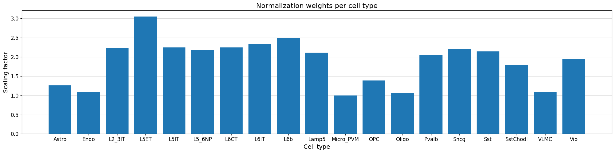
Peak normalization#
We can normalize our peak values based on the variability of the top peak heights per cell type using the crested.pp.normalize_peaks() function.
This function applies a normalization scalar to each cell type, obtained by comparing per cell type the distribution of peak heights for the maximally accessible regions which are not specific to any cell type.
crested.pp.normalize_peaks(adata, top_k_percent=0.03)
2026-02-17T16:22:29.346358+0100 INFO Filtering on top k Gini scores...
2026-02-17T16:22:33.657138+0100 INFO Added normalization weights to adata.obsm['weights']...
| chr | start | end | target_start | target_end | split | |
|---|---|---|---|---|---|---|
| region | ||||||
| chr9:76566142-76568190 | chr9 | 76566142 | 76568190 | 76566666 | 76567666 | train |
| chr5:98328510-98330558 | chr5 | 98328510 | 98330558 | 98329034 | 98330034 | train |
| chr5:98347819-98349867 | chr5 | 98347819 | 98349867 | 98348343 | 98349343 | train |
| chr13:34635167-34637215 | chr13 | 34635167 | 34637215 | 34635691 | 34636691 | train |
| chr13:34642109-34644157 | chr13 | 34642109 | 34644157 | 34642633 | 34643633 | train |
| ... | ... | ... | ... | ... | ... | ... |
| chr13:34344270-34346318 | chr13 | 34344270 | 34346318 | 34344794 | 34345794 | train |
| chr5:98166140-98168188 | chr5 | 98166140 | 98168188 | 98166664 | 98167664 | train |
| chr5:98166667-98168715 | chr5 | 98166667 | 98168715 | 98167191 | 98168191 | train |
| chr13:34344974-34347022 | chr13 | 34344974 | 34347022 | 34345498 | 34346498 | train |
| chr5:98185712-98187760 | chr5 | 98185712 | 98187760 | 98186236 | 98187236 | train |
48089 rows × 6 columns
We can visualize the normalization factor for each cell type using the crested.pl.qc.normalization_weights() function to inspect which cell type peaks were up/down weighted.
%matplotlib inline
crested.pl.qc.normalization_weights(adata, title="Normalization weights per cell type")
Subset to specific regions#
Like in the main tutorial, we also create a subset of specific regions. We found that double fine-tuning works better than single-round on either all or the specific peaks. This is the same subset as used in the default tutorial.
adata_filtered = crested.pp.filter_regions_on_specificity(adata, gini_std_threshold=1.0, inplace=False)
2026-02-17T16:23:22.003894+0100 INFO After specificity filtering, kept 90995 out of 543847 regions.
Load in model#
We load in the Borzoi model’s weights in its architecture, with one change - the input length. All of Borzoi’s layers are width-independent, so the length can be set to any value divisible by the internal bin size (128bp).
target_length is set to the total number of output bins (64 bins of 32bp makes 2048bp output), since no cropping is needed when predicting local features.
num_classes is set to the original size simply so that there are no weight shape mismatches when loading the initial weights; the head created based on num_classes will be replaced by a new head for the number of cell types we’d like to predict below.
# Create default Borzoi architecture, with shrunk input size and target_length
base_model_architecture = crested.tl.zoo.borzoi(seq_len=2048, target_length=2048//32, num_classes=2608)
To load in the weights, we can’t directly load the model from the .keras file, since that fixes the input length at the previously set value (524288bp). However, we can extract the model.weights.h5 file containing only the weights and use that.
# Load pretrained Borzoi weights
model_file, _ = crested.get_model("Borzoi_mouse_rep0")
# Put weights into base architecture
with zipfile.ZipFile(model_file) as model_archive, tempfile.TemporaryDirectory() as tmpdir:
    model_weights_path = model_archive.extract("model.weights.h5", tmpdir)
    base_model_architecture.load_weights(model_weights_path)
Now that we have the base model with the adjusted input shape, we need to adjust the final layers to return a value for each cell type per region, instead of per-bin values. Therefore, we drop the final head, add a flatten layer after the model’s final embedding, and add a new head predicting adata.n_obs values.
# Replace track head by flatten+dense to predict single vector of scalars per region
## Get last layer before head
current = base_model_architecture.get_layer("final_conv_activation").output
## Flatten and add new layer
current = keras.layers.Flatten()(current)
current = keras.layers.Dense(adata.n_obs, activation="softplus", name="dense_out")(current)

# Turn into model
model_architecture = keras.Model(inputs=base_model_architecture.inputs, outputs=current, name="Borzoi_scalar")
print(model_architecture.summary())
Model training#
Parameters#
The DataModule and TaskConfig let you set standard training parameters, like batch size and learning rate.
We use the same parameters as with peak regression in the default tutorial, except for a lower learning rate to match the fact that we are starting from a pre-trained model.
datamodule = crested.tl.data.AnnDataModule(
    adata,
    genome=genome,
    batch_size=32,  # lower this if you encounter OOM errors
    max_stochastic_shift=3,  # optional augmentation
    always_reverse_complement=True,  # default True. Will double the effective size of the training dataset.
)
optimizer = keras.optimizers.Adam(learning_rate=1e-5)
loss = crested.tl.losses.CosineMSELogLoss(max_weight=100, multiplier=1)
metrics = [
    keras.metrics.MeanAbsoluteError(),
    keras.metrics.MeanSquaredError(),
    keras.metrics.CosineSimilarity(axis=1),
    crested.tl.metrics.PearsonCorrelation(),
    crested.tl.metrics.ConcordanceCorrelationCoefficient(),
    crested.tl.metrics.PearsonCorrelationLog(),
]

config = crested.tl.TaskConfig(optimizer, loss, metrics)
print(config)
TaskConfig(optimizer=<keras.src.optimizers.adam.Adam object at 0x1469e0eb4ec0>, loss=CosineMSELogLoss: {'name': 'CosineMSELogLoss', 'reduction': 'sum_over_batch_size', 'max_weight': 100}, metrics=[<MeanAbsoluteError name=mean_absolute_error>, <MeanSquaredError name=mean_squared_error>, <CosineSimilarity name=cosine_similarity>, <PearsonCorrelation name=pearson_correlation>, <ConcordanceCorrelationCoefficient name=concordance_correlation_coefficient>, <PearsonCorrelationLog name=pearson_correlation_log>, <ZeroPenaltyMetric name=zero_penalty_metric>])
Finetune on full peak set#
By default:
The model will continue training until the validation loss stops decreasing for 10 epochs with a maximum of 100 epochs.
Every best model is saved based on the validation loss.
The learning rate reduces by a factor of 0.25 if the validation loss stops decreasing for 5 epochs.
# setup the trainer
trainer = crested.tl.Crested(
    data=datamodule,
    model=model_architecture,
    config=config,
    project_name="biccn_borzoi_atac",
    run_name="testrun",
    logger="wandb",
)
# train the model
trainer.fit(epochs=10)
Further finetuning on specific regions#
We found that finetuning on the full peak set, then on the filtered peak set improved performance over training only on either set. Therefore, we’ll filter the peaks to keep only cell type-specific peaks and further finetune the model.
datamodule = crested.tl.data.AnnDataModule(
    adata_filtered,
    genome=genome,
    batch_size=32,  # lower this if you encounter OOM errors
    max_stochastic_shift=3,  # optional augmentation
    always_reverse_complement=True,  # default True. Will double the effective size of the training dataset.
)
optimizer = keras.optimizers.Adam(learning_rate=5e-5)
loss = crested.tl.losses.CosineMSELogLoss(max_weight=100, multiplier=1)
metrics = [
    keras.metrics.MeanAbsoluteError(),
    keras.metrics.MeanSquaredError(),
    keras.metrics.CosineSimilarity(axis=1),
    crested.tl.metrics.PearsonCorrelation(),
    crested.tl.metrics.ConcordanceCorrelationCoefficient(),
    crested.tl.metrics.PearsonCorrelationLog(),
    crested.tl.metrics.ZeroPenaltyMetric(),
]

config = crested.tl.TaskConfig(optimizer, loss, metrics)
print(config)
TaskConfig(optimizer=<keras.src.optimizers.adam.Adam object at 0x1469e0d60910>, loss=CosineMSELogLoss: {'name': 'CosineMSELogLoss', 'reduction': 'sum_over_batch_size', 'max_weight': 100}, metrics=[<MeanAbsoluteError name=mean_absolute_error>, <MeanSquaredError name=mean_squared_error>, <CosineSimilarity name=cosine_similarity>, <PearsonCorrelation name=pearson_correlation>, <ConcordanceCorrelationCoefficient name=concordance_correlation_coefficient>, <PearsonCorrelationLog name=pearson_correlation_log>, <ZeroPenaltyMetric name=zero_penalty_metric>])
model_architecture = keras.models.load_model("biccn_borzoi_atac/testrun/checkpoints/03.keras", compile=False)
# setup the trainer
trainer = crested.tl.Crested(
    data=datamodule,
    model=model_architecture,
    config=config,
    project_name="biccn_borzoi_atac",
    run_name="testrun_ft",
    logger="wandb",
)
# train the model
trainer.fit(epochs=5)
Evaluate model#
We’ll evaluate both the finetuned and further finetuned models, and compare against DeepBICCN2, a dilated CNN model from our registry trained on the same dataset (closely matching the main tutorial).
model = keras.models.load_model("biccn_borzoi_atac/testrun/checkpoints/03.keras", compile=False)
model_ft = keras.models.load_model("biccn_borzoi_atac/testrun_ft/checkpoints/01.keras", compile=False)
# Add predictions for model checkpoint to the adatas
adata.layers["Once finetuned"] = crested.tl.predict(adata, model).T
adata.layers["Double finetuned"] = crested.tl.predict(adata, model_ft).T

# Copy predictions for specific peaks
adata_filtered.layers["Once finetuned"] = adata.layers["Once finetuned"][:, adata.var_names.get_indexer(adata_filtered.var_names)]
adata_filtered.layers["Double finetuned"] = adata.layers["Double finetuned"][:, adata.var_names.get_indexer(adata_filtered.var_names)]
# Load in the DeepBICCN2 model
model_file_db2, output_names_db2 = crested.get_model('deepbiccn2')
deepbiccn2 = keras.models.load_model(model_file_db2, compile=False)
# Get resized anndatas to deal with the slightly different input size
adata_2114 = crested.pp.change_regions_width(adata, 2114, inplace=False)
# Predict values
adata.layers["DeepBICCN2"] = crested.tl.predict(adata_2114, deepbiccn2).T
adata_filtered.layers["DeepBICCN2"] = adata.layers["DeepBICCN2"][:, adata.var_names.get_indexer(adata_filtered.var_names)]
del adata_2114
4245/4249 ━━━━━━━━━━━━━━━━━━━━ 0s 17ms/step
4249/4249 ━━━━━━━━━━━━━━━━━━━━ 121s 22ms/step
# Save the anndata with these predictions
adata.write_h5ad("crested/mouse_cortex_preds.h5ad")
# Read in data again
adata = ad.read_h5ad("crested/mouse_cortex_preds.h5ad")
adata_filtered = crested.pp.filter_regions_on_specificity(adata, gini_std_threshold=1.0, inplace=False)
2026-02-17T16:41:31.725655+0100 INFO Lazily importing module crested.pp. This could take a second...
2026-02-17T16:41:37.760591+0100 INFO After specificity filtering, kept 90995 out of 543847 regions.
Many of the plotting functions in the crested.pl module can be used to visualize these model predictions.
# Define a dataframe with test set regions
test_df = adata.var[adata.var["split"] == "test"]
test_df_ft = adata_filtered.var[adata_filtered.var["split"] == "test"]
test_df
| chr | start | end | target_start | target_end | split | |
|---|---|---|---|---|---|---|
| region | ||||||
| chr1:3094031-3096079 | chr1 | 3094031 | 3096079 | 3094555 | 3095555 | test |
| chr1:3094696-3096744 | chr1 | 3094696 | 3096744 | 3095220 | 3096220 | test |
| chr1:3111400-3113448 | chr1 | 3111400 | 3113448 | 3111924 | 3112924 | test |
| chr1:3112760-3114808 | chr1 | 3112760 | 3114808 | 3113284 | 3114284 | test |
| chr1:3118972-3121020 | chr1 | 3118972 | 3121020 | 3119496 | 3120496 | test |
| ... | ... | ... | ... | ... | ... | ... |
| chrX:21361135-21363183 | chrX | 21361135 | 21363183 | 21361659 | 21362659 | test |
| chrX:21388522-21390570 | chrX | 21388522 | 21390570 | 21389046 | 21390046 | test |
| chrX:21392726-21394774 | chrX | 21392726 | 21394774 | 21393250 | 21394250 | test |
| chrX:21427413-21429461 | chrX | 21427413 | 21429461 | 21427937 | 21428937 | test |
| chrX:21433814-21435862 | chrX | 21433814 | 21435862 | 21434338 | 21435338 | test |
58874 rows × 6 columns
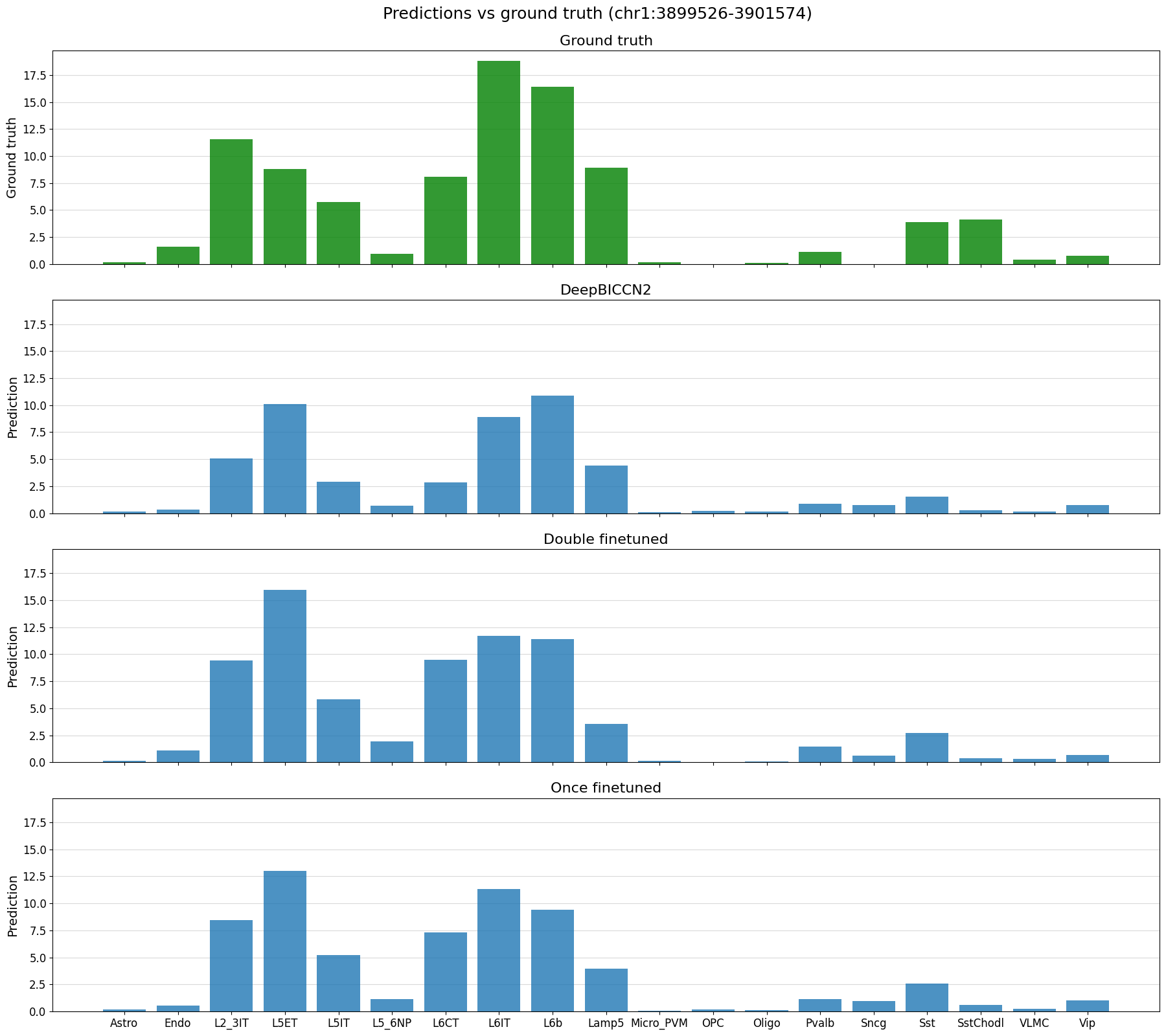
# plot predictions vs ground truth for a random region in the test set defined by index
%matplotlib inline
idx = 22
region = test_df_ft.index[idx]
print(region)
crested.pl.region.bar(adata_filtered, region, suptitle=f"Predictions vs ground truth ({region})")
chr1:3899526-3901574
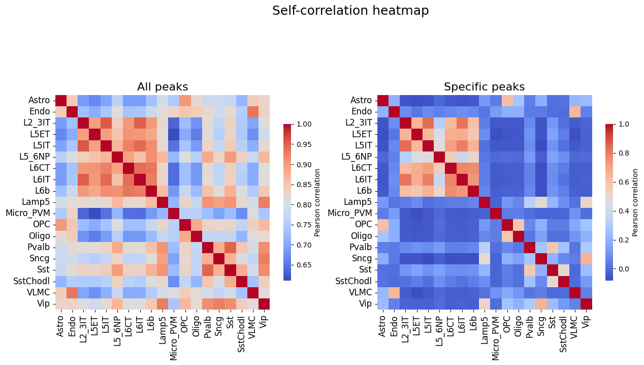
# Self-correlation values of all peaks and specific peaks, upper bound on the correlations between truth and predictions
%matplotlib inline
fig, axs = plt.subplots(1, 2, figsize = (15, 8))
crested.pl.corr.heatmap_self(
    adata,
    title="All peaks",
    show=False,
    ax=axs[0],
    cbar_kws={'shrink': 0.5}
)
crested.pl.corr.heatmap_self(
    adata_filtered,
    title="Specific peaks",
    suptitle="Self-correlation heatmap",
    ax=axs[1],
    show=False,
    cbar_kws={'shrink': 0.5}
)
plt.show()
2026-02-17T16:43:27.543253+0100 WARNING Using keyword argument layout does not do anything when passing a pre-existing axis.
2026-02-17T16:43:27.640792+0100 WARNING Using keyword argument layout does not do anything when passing a pre-existing axis.
(<Figure size 1500x800 with 4 Axes>,
 <Axes: title={'center': 'Specific peaks'}>)
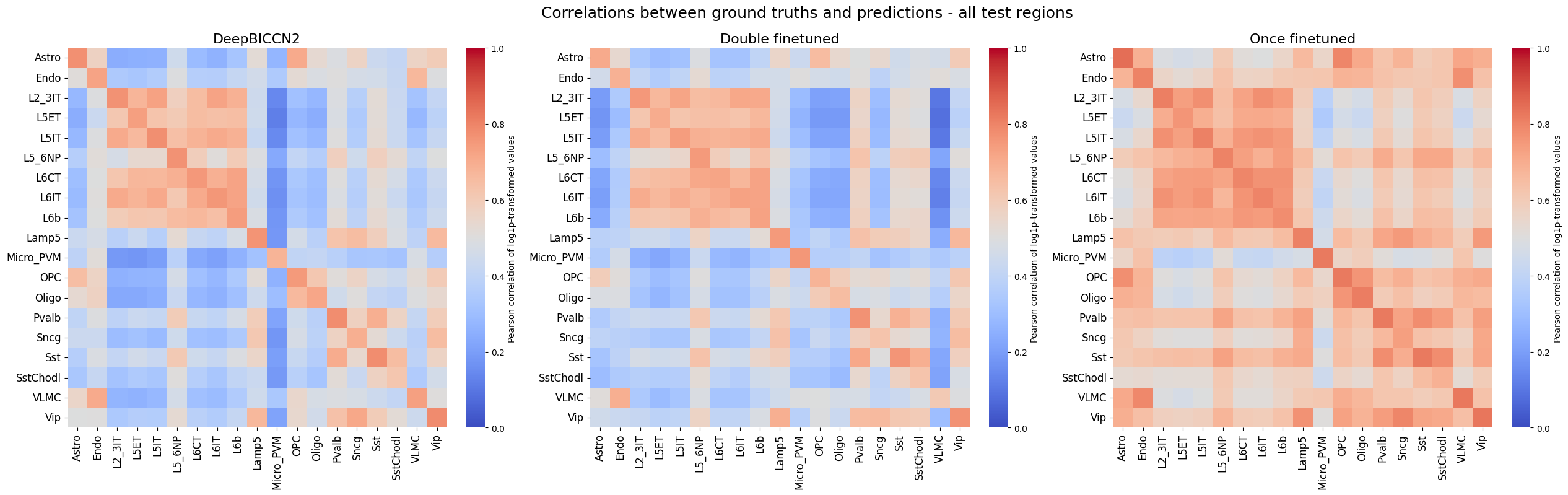
%matplotlib inline
crested.pl.corr.heatmap(
adata,
split="test",
suptitle="Correlations between ground truths and predictions - all test regions",
log_transform=True,
vmin = 0,
vmax = 1,
)
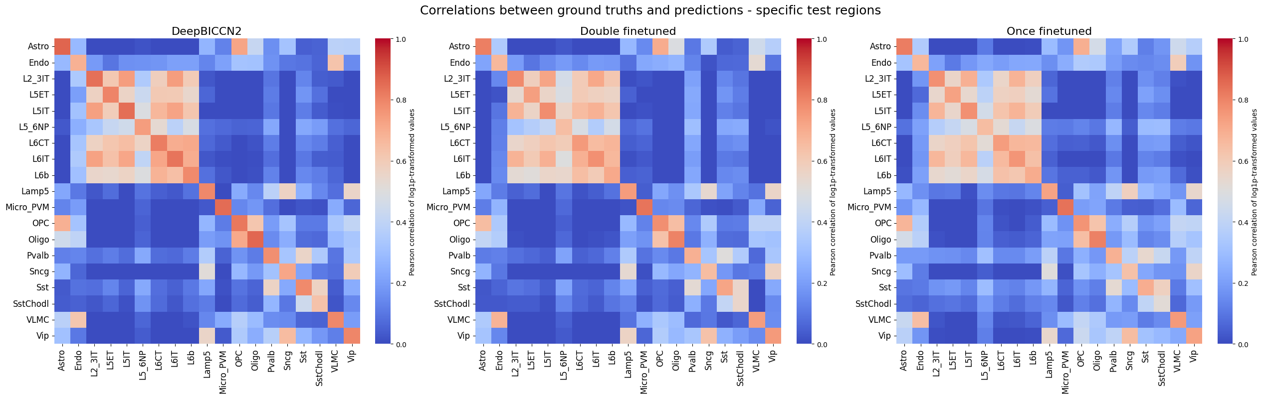
crested.pl.corr.heatmap(
adata_filtered,
split="test",
suptitle="Correlations between ground truths and predictions - specific test regions",
log_transform=True,
vmin = 0,
vmax = 1,
)
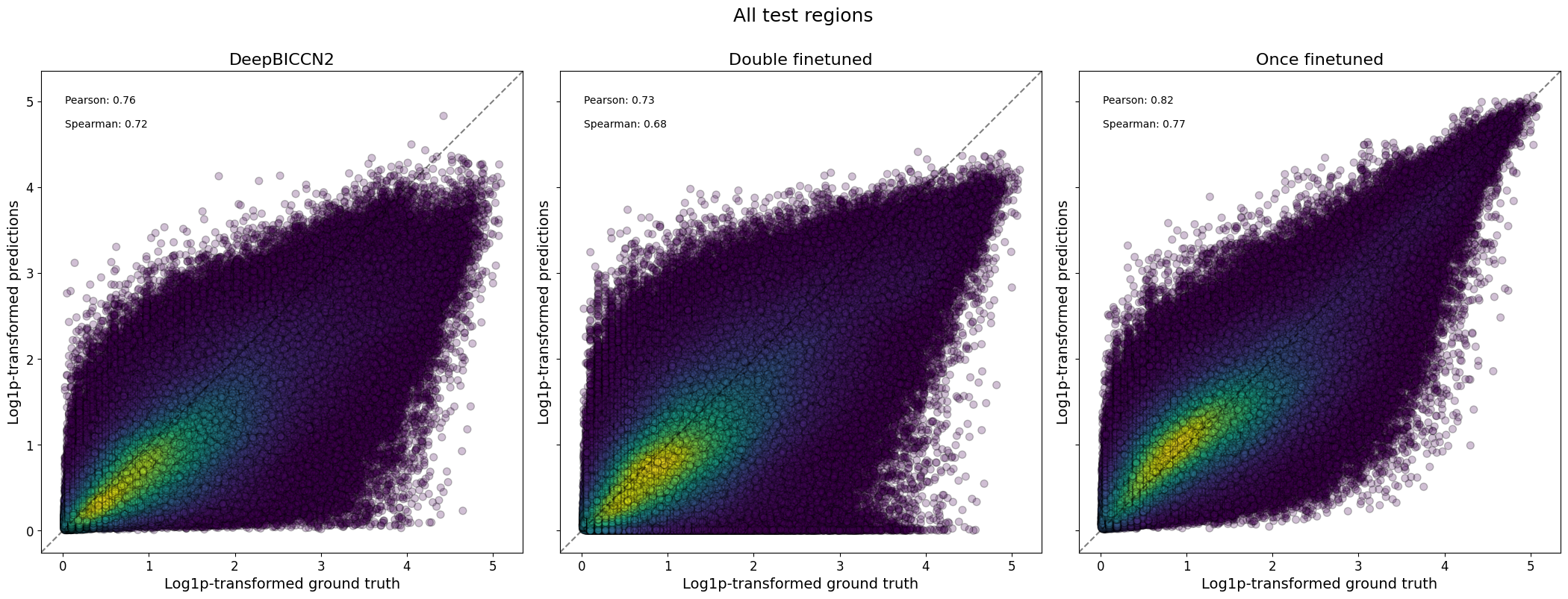
%matplotlib inline
crested.pl.corr.scatter(
adata,
split="test",
suptitle="All test regions",
log_transform=True,
density_indication=True,
identity_line=True,
square=True
)
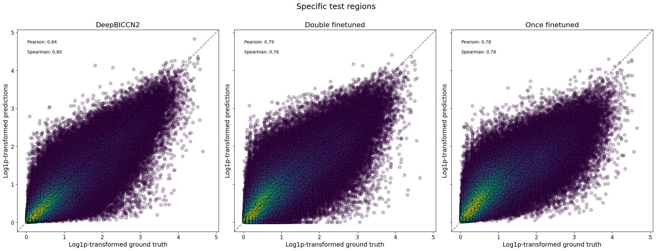
crested.pl.corr.scatter(
adata_filtered,
split="test",
suptitle="Specific test regions",
log_transform=True,
density_indication=True,
identity_line=True,
square=True
)
2026-02-17T16:45:22.573983+0100 INFO Plotting density scatter for all targets and predictions, models: ['DeepBICCN2', 'Double finetuned', 'Once finetuned'], split: test
2026-02-17T16:46:41.194634+0100 INFO Plotting density scatter for all targets and predictions, models: ['DeepBICCN2', 'Double finetuned', 'Once finetuned'], split: test
%matplotlib inline
model_order = ["DeepBICCN2", "Once finetuned", "Double finetuned"]
fig, axs = plt.subplots(1, 2, figsize=(15, 8))
crested.pl.corr.violin(
    adata,
    ax=axs[0],
    title="All peaks",
    suptitle="Per-class correlations compared between models and datasets",
    plot_kws={'order': model_order},
    show=False,
)
crested.pl.corr.violin(adata_filtered, ax=axs[1], title="Specific peaks", plot_kws={'order': model_order}, show=False)
plt.show()
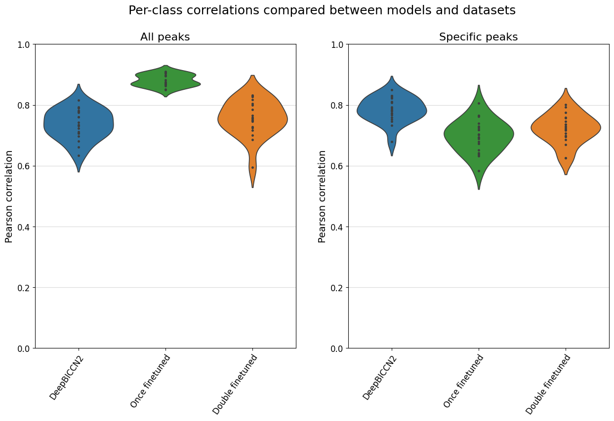
Here, we see that the fine-tuned models generally stack up very comparably to the CNN-based models on this dataset, but that they don’t have an edge.
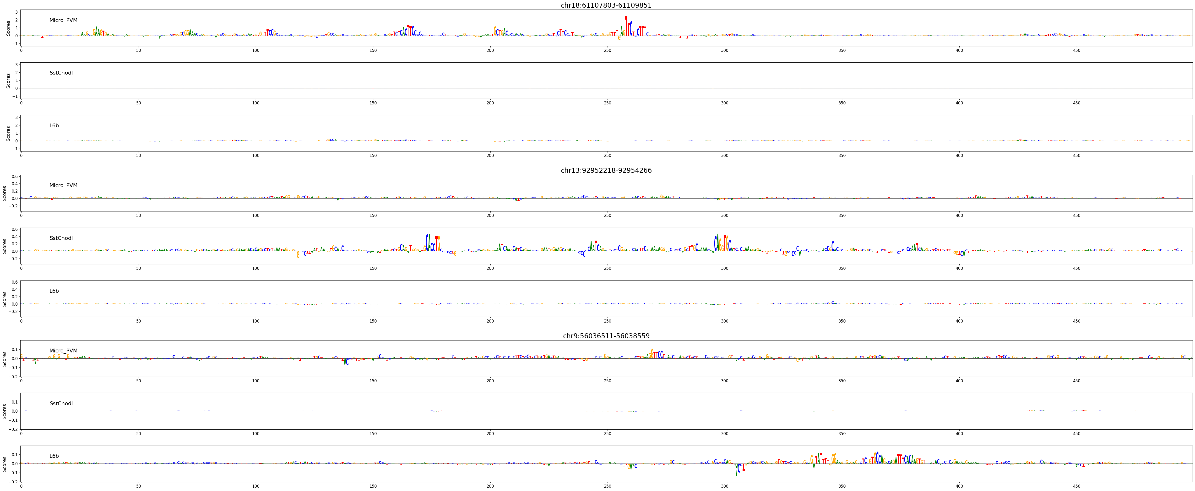
Besides looking at prediction scores, we can also use these models to explain the features in the sequence that contributed to predicted accessibility in a certain cell type.
Here, we’ll look at three regions, expected to be active in microglia (Micro_PVM), Sst/Chodl GABAergic neurons (SstChodl), or in layer 6b glutamatergic neurons (L6b) respectively.
regions_of_interest = [
    "chr18:61107803-61109851",
    "chr13:92952218-92954266",
    "chr9:56036511-56038559",
]
classes_of_interest = ["Micro_PVM", "SstChodl", "L6b"]
class_idx = list(adata.obs_names.get_indexer(classes_of_interest))

scores, one_hot_encoded_sequences = crested.tl.contribution_scores(
    regions_of_interest,
    target_idx=class_idx,
    model=model_ft,
)
2026-02-17T16:52:53.490277+0100 INFO Calculating contribution scores for 3 class(es) and 3 region(s).
# Plot attribution scores
crested.pl.explain.contribution_scores(
    scores,
    one_hot_encoded_sequences,
    sequence_labels=regions_of_interest,
    class_labels=classes_of_interest,
    zoom_n_bases=500,
    title_fontsize=20,
)